In my research I recently needed into discrete control and started to dive into Markov Decision Processes (MDP) and Partial Observable Markov Decision Processes (POMDP). At a first glance just these terms may seem sophisticated to the naked eye, but I will show that these two are actually very powerful tools to model decision-making and therefore implement discrete control paradigms.

Unfortunately this topic is usually covered with plenty of math in textbook which leaves poor grad students like me with converting the math into usable code. In this and the following articles I want to share some experience I have gained so far in implementing Markov Decision processes.

In order to make this hands-on and not just dump math at you, I will provide example code in Python/numpy, with all algorithms implemented from scratch, and explain the guts using the formulas and the implementation.

Background: Decision Processes

Suppose you are confronted with making a decision, you are usually confronted with a number of possible actions you can perform that will have some effects on your environment and each decision has some benefit or cost associated with it. The effects of the immediate actions are usually easy to see, however the long-term consequences are hard to predict. Coming up with a general model for decisions is non-trivial because making the decisions can depend on many factors of the environment; especially other people in your environment; your beliefs, your observations, your capabilities, and the questions you try to answer with your model. To get a sense of this claim the reader is referred to the large domain of Game Theory that actually comes up with many models for “toy-problems”. Unfortunately, the questions Game Theoretic approaches seek to address are usually different from what someone needs to build a decision process to model a control problem.

For example, consider yourself in a clothing store. Your initial objective is to buy nice clothing, and you may consider going back to the store if you like it. The shelves in the store have some items to choose from and some cost associated with it. Suppose you like the friendly lady in the store, and you do not want to look old-fashioned in front of her. Soon your objectives, available actions and system boundaries change, and you need to take her views and beliefs into consideration. Worse, consider belief nesting: What if she thinks that I think she might think… in shortcoming up with a realistic model which jacket to choose or paying subsequent visits to the store is not easy.

When approaching technical control problems, we need to sacrifice some aspects of real life we deem less important. The first step in simplification is to close the problem space, by only considering…

• A finite number of states of the environment.
• A finite number of actions to choose from.
• A finite number of effects on the environment.
• Associating defined cost with each action in each state.

Making the above simplifications eases the process a lot. Since a decision-making process involves a sequence of decisions. Another huge simplification is to only consider the effects of the last decision made, this is called Markov assumption.

Making the above assumptions opens the door to use two standard frameworks for modelling decision processes, namely the Markov Decision Process (MDP) and the Partial Observable Markov Decision Process (POMDP) which will be covered in part two of the article.

Markov Decision Process (MDP)

A Markov Decision Process is a simple stochastic control process that satisfies the assumptions and model of the previous topics. It is well suited for problems where you can model the entire environment as states and make them visible to your agent (i.e., the entity making the decisions). In addition most solution algorithms that compute the control action assume that the definition of states, cost and actions and is fixed and time-invariant. That means that the reward for a particular action in a particular state does not change from time to time. Ok let’s get dirty and formalize this stochastic tool:

• $mathbb{S}$ is the finite set of states
• $mathbb{A}$ is a finite set of actions, with $mathbb{A}_{s} subseteq mathbb{A}$ being the available actions in a particular State $s in mathbb{S}$
• $ext{P}_a(s, s_n)$ the probability that Action $a in mathbb{A}$ in State $s in mathbb{S}$ leads to State $s_n in mathbb{S}$. Because most solution algorithms consider this function to be time-invariant, it can be easily modeled as a family of matrices, one matrix per action.
• $ext{R}_a(s, s_n)$ is the expected immediate reward (or cost) after the transition from State $s in mathbb{S}$ to State $s_n in mathbb{S}$ given a particular action. If the rewards are time-invariant, this function can be represented as a family of matrices as well.

An MDP is fully specified when those functions are given. There are two key control problems that can be answered with MDPs.

• What is the optimal action to advance into any other state?
• What is the optimal plan to for a finite number of transitions?

Having a complete view of the expected rewards, the states of the environment and the current state, the computation of one step and a finite number of steps is a straightforward optimization problem. Before digging into the math, let’s consider a simple example. A model how to become one of the rich and famous (this was originally proposed by Andreas Krause at CALTECH University, see references).

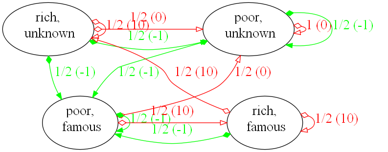
In this model there are two actions. First we can spend money on advertising to become famous (f) or save our money to become rich (r). Depending on the state we are in we have different chances of becoming famous or rich. In the diagram the red lines show the effects of advertise action, the green lines the save action. Each edge is labelled with the transition probability and the associated reward or (cost for negative numbers). Assume being poor (p) and unknown (u) and deciding to advertise (green lines). Then we have a 50-50 of becoming poor and famous or remain poor and unknown; in both cases we have a cost of 1. The decision to advertise yields a cost of one in both cases. From this simple model we can construct our mathematical model.

• $mathbb{S}$ = $lbrace pu, pf, ru, rf brace$
• $mathbb{A}$ = $lbrace ext{advertise}, ext{save} brace$
• $ext{P}$ and $ext{R}$ are initialized as shown in the graph.

Python and numpy support easy initialization of matrices and arrays. The complete model definition is shown in the source below.

import numpy

# definition of states
S = numpy.array(['pu', 'pf', 'ru', 'rf'])
# definition of actions (just for output
# we will work with int indices of them
A = numpy.array(['advertise', 'save'])

# definition of expected rewards
R = [ numpy.array( # advertise
    [#pu   pf   ru   rf 
     [-1.0, -1.0, 0.0, 0.0], # pu
     [ 0.0, -1.0, 0.0, 0.0], # pf
     [-1.0, -1.0, 0.0, 0.0], # ru
     [ 0.0, -1.0, 0.0, 0.0], # rf
    ]),
    numpy.array( # save
    [#pu   pf   ru   rf 
     [0.0, 0.0, 0.0, 0.0],  # pu
     [0.0, 0.0, 0.0, 10.0], # pf
     [0.0, 0.0, 10,  0.0],  # ru
     [0.0, 0.0, 10,  10],   # rf
    ])]

# definition of transition probabilities
T = [numpy.array( # advertise
    [#pu   pf   ru   rf 
     [0.5, 0.5, 0.0, 0.0], # pu
     [0.0, 1.0, 0.0, 0.0], # pf
     [0.5, 0.5, 0.0, 0.0], # ru
     [0.0, 1.0, 0.0, 0.0], # rf
    ]),
    numpy.array( # save
    [#pu   pf   ru   rf 
     [1.0, 0.0, 0.0, 0.0], # pu
     [0.5, 0.0, 0.0, 0.5], # pf
     [0.5, 0.0, 0.5, 0.0], # ru
     [0.0, 0.0, 0.5, 0.5], # rf
    ])]

Based on that model, how do we derive an optimal policy that maximizes the reward in each step? The beauty about this example is that the transitions are actually stochastic and therefore the expected rewards. In this example the rewards are fully defined, but for many real-world problems these rewards are not fully defined upfront or distributed with an unknown distribution. In that case we should instead explore the world and update our model based on the observations. A tool that enables this type of online learning is reinforcement learning specifically a Q-learner. In a nutshell the Q-learner learns a function that assigns utility to making a particular action in state s for future states. The beauty about a Q-learner is its ability to learn transition probabilities and rewards from observations. Its parameters give control about how much an agent should plan ahead when making a decision and how fast to learn. Formally the learning is performed as follows.

$$ext{Q}(s_t, a_t) := ext{Q}_n(s_t, a_t) (1-alpha) + alpha (r + gamma ext{argmax}_{a} ext{Q}(s_{t+1}, a)$$

The formula is straightforward. The individual parameters are as follows:

• $ext{Q}_n(s_t, a_t)$: the old utility value of the current state $s_t$, given the action $a_t$.
• $ext{Q}(s_{t+1}, a_t)$: Is the expected utility of traversing into state $s_{t+1}$ by committing action $a_t$. Note this utility is approximated from past observations and is therefore defined.
• $alpha$: The learning rate. It specifies how much the agent learns from the current observation. A value of 0 means it learns nothing, a value of 1 would only consider the most recent observation.
• $gamma$: The discount factor. It specifies the importance of future rewards and therefore the planning horizon of the agent. A factor of 0 makes the agent opportunistic and only lets it consider the next state. A value of 1 would make it strive for long-term results. Note that larger values than 1 make the learning instable.
• $r$ is the observed reward after committing action $a_t$.

One question to answer is now how to make the agent explore the state space to approximate the utility of actions in particular states. A naïve approach is to just randomly select an available action in each state; this would probably exercise most of the action/state configurations but yields suboptimal results since we are already controlling something while learning. A slight optimization is to stochastically select the next action based on the observed utilities, but also this could push the learning into a local optimum. Another approach is to take a tool from thermodynamics and model the “stupidity” of the agent using the Boltzmann distribution. The Boltzmann distribution originally was used to model the velocity distributions of particles in gases based on the temperature. Instead of modeling particles, we model individual decisions based on an underlying distribution of utilities. We (mis-)use the “temperature” parameter of the distribution to model stupidity. A value approaching 0 would generate stochastic decisions following the distribution of utilities; a higher value would smooth the underlying distribution and distribute the values more uniformly. Putting that into context of making decisions, a high value would generate decisions alike the shopping behaviour of a young rich college girl (no offence intended) and a low value would model the shopping behaviour of a retiree that is trying to get the most of his pension (no offence intended either).

$$p_i := rac{e^{rac{u_i}{k}}}{sum_j e^{rac{u_j}{k}}}$$

The components of the Boltzmann distribution are as follows:

• $k$ is the temperature parameter
• $u_i$ is some measure (e.g., utility or success probability) for the action $i$
• $p_i$ is the success probability for an action $i$ given the temperature $k$

A neat thing, when incorporating the Boltzmann distribution into our model we can make it dynamic and become more conservative about the decisions made by decreasing the temperature parameter within each step, the more we learn about the world. Ok let’s look at the implementation of the Boltzmann distribution in numpy.

    @staticmethod
    def BOLTZMANN(k, Qs):
        '''Computes the Boltzmann distribution
        for doing something "stupid".
        @param k: temperature (aka stupidity)
        @param Qs: array of q values of the
        current state.
        '''
        # compute e^(q)/k for all actions
        Es = numpy.exp(Qs/k)
        
        # [x_j : e^[ q(a_j,s)/k ] / 
        # [sum_j e^[q(a_j, s)/k]]]
        return Es/numpy.sum(Es)

Numpy supports element-wise array operations which makes the implementation straightforward and short. The function returns an array of probabilities for making decisions.

The next building block we need is a random number generator that can generate the decisions based on a discrete probability distribution. Unfortunately, neither numpy nor Python provide a function that performs this mapping. However, one can easily implement their own distribution by leveraging the uniform(0,1) distribution. The technique works as follows:

1. Pick a random number from uniform(0,1)
2. Stick it into the quantile-function (i.e. the inverse cumulative probability distribution function) of the target distribution
3. Take this value and enjoy your custom random process.

The above approach is also referred to as Smirnoff-transformation. The quantile function of our array of probabilities is a mapping from a probability to an index. This can be implemented by computing the cumulative distribution function (CDF) of the probabilities on the fly and comparing it to the input probability. Once the CDF is larger than the probability we can take the previous index. If you look at the following code this procedure becomes more obvious.

    @staticmethod
    def DECIDE(distro):
        ''' pick a state at random given a
        probability distribution over
        discrete states
        @param distro: the prob. distribution'''
        # make decision
        r = numpy.random.rand()
        tmp = 0
        for a in xrange(len(distro)):
            tmp += distro[a]
            if r < tmp:
                # decision made
                break
        return a

Ok putting all the building blocks together, we can implement iteration as follows.

    def iterate(self):
        '''Performs one action in the current
        state and updates the q-values'''
        
        # decide which action to take based
        # on Boltzmann distro of q-values of
        # the current state
        dist = self.BOLTZMANN(self.k, self.Qs[self.cs])
        
        # normalise
        dist /= numpy.sum(dist)
        
        # pick a random action
        a = self.DECIDE(dist)
        
        # decide new state based on transition
        # probabilities
        tsp = self.T[a][self.cs,:]
        newState = self.DECIDE(tsp)
        
        # compute reward
        r = self.R[a][self.cs, newState]
        
        self.Qs[self.cs, a] = (
             self.Qs[self.cs, a] * (1.0 - self.alpha) +
             self.alpha * (r + self.gamma * numpy.max(self.Qs[newState])))
        
        # update strategy for state
        self.cs = newState

The model parameters are the same as described above in the initialization. The matrix Qs models the utilities of particular states given an action. When invoking this method we can adjust the learning parameters which are gamma, the discount factor that controls the long-term outlook of the learner, alpha, the learning rate that weights the observations made, and k which models the stupidity of making decisions. In the sample code only k is reduced in a linear fashion with each learning step.

The optimal policy for this model is to advertise in the poor-unknown state and save in all other states until you are rich and famous.

Conclusion

In this first part, I introduced stochastic Markov Decision processes and exemplified the learning of such processes with stochastic rewards using a Q-learner. The exploration of the process is controlled using a dynamic Boltzmann distribution that makes the learner make more conservative decisions the more it knows about the environment. All the artefacts of this model were implemented in python using numpy. Although python is an interpreted language, by leveraging the performance of numpy’s array operations we can implement an affordable learner. The reader should note that there are more efficient policy iteration methods for MDPs if the rewards are fixed (i.e., value-iteration and policy iteration), however this is not generally the case. Furthermore the model presented here may not make you rich, there are other ways of getting rich in practice :D. I hope you enjoyed this part of tutorial.

• Sample Code (provided under the terms of the LGPL)
• Q-Learning
• Boltzmann Distribution
• Smirnoff Transformation
• Andreas Krauses Course notes, dead link in 2025

---

Cross posted from m old blog

Published: 2010-02-19
Updated  : 2025-10-04
Not a spam bot? Want to leave comments or provide editorial guidance? Please click any of the social links below and make an effort to connect. I promise I read all messages and will respond at my choosing.